VIX Dispersion (Thrasher 2017) — Paper-Faithful Signal
📄 docs
🌊 Thrasher VIX Dispersion Signal Active — 20-day StdDev compressed below 15th percentile.
Paper backtest (2006-2016, 52 signals): avg max +34.3%, median +23.0% over next 15 trading days. Single indicator, no other filters. Forward window: 15 trading days from signal.
Our reproduction (2016-2026, 48 signals): avg max +22.7%, median +14.2% — edge degraded post-2016. 8.2% of signals followed by paper's 30%+ 5-day spike vs paper's implied >50%. Methodology may be regime-dependent.
VIX Signal
—
StdDev(20) vs 15th pct
VIX 20-Day StdDev
—
threshold: —
StdDev Percentile
—
vs full history
VVIX Signal (secondary)
—
15th pct of VVIX StdDev(20)
VIX 20-Day Standard Deviation vs Threshold (1Y) — Signal Days Marked
Blue line = VIX 20d StdDev. Dashed = 15th-percentile threshold (adaptive to full history). Red markers = signal-fired days (StdDev ≤ threshold with 10-day dedup).
Spot + M1 + M2, including first contract past 60 DTE. Dot color = contract identity (shared with spread charts below).
M1 − Spot Spread (Front Month vs VIX)
M2 − Spot Spread (2nd Month vs VIX)
M1 − M2 Spread (Short-End Contango, Raw Points)
Raw vol points (M2 settle − M1 settle). M1/M2 identity rolls on the Wednesday exactly 14 calendar days before the front contract's expiry — earlier than the actual-expiry roll used in the M1/M2 vs Spot charts above.
Line color flips at each contract roll — segments are colored by which contract was the M1/M2 on that date, matching dot colors on the short-end curve above and the full term structure chart at top.
KEY RATES—
BREAKEVEN INFLATION—
MACRO CONTEXT—
EQUITY REPO—
FedWatch Probability Table
Calendar Spread Matrix (bp)
Layer 1 — Policy Anchors
Target Range
—
—
IORB
—
—
ON RRP Rate
—
—
Layer 2 — Market Reality
EFFR
—
—
SOFR
—
—
SOFR − EFFR
—
cash↔collateral regime gauge
EFFR vs SOFR — 90d
Layer 3 — Plumbing Flows
ON RRP Balance
—
—
Reserves
—
—
TGA
—
—
ON RRP Balance — 180d
Reserves & TGA — 365d
Source: FRED CSV endpoints (EFFR/SOFR/IORB/RRPONTSYAWARD/RRPONTSYD/DFEDTARU/DFEDTARL/WRESBAL/WTREGEN/DTB4WK/DTB3/DTB6).
Refresh: 7AM ET weekdays. Framing: Conks · conks.plumbing.
Loading…
Select a term on the left.
Definitions written by Jarvis from primary references. Framing draws on
Conks · conks.plumbing — wording is ours.
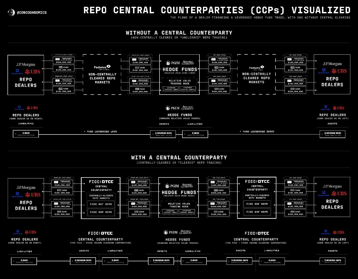
Repo CCPs — Source Diagram
The flows of a dealer financing a leveraged hedge-fund trade, with and without central clearing.
Compares non-cleared bilateral repo (top) — Dealer ↔ Fedwire ↔ HF ↔ Fedwire ↔ Dealer —
against centrally-cleared repo (bottom) — Dealer ↔ FICC/DTCC ↔ HF ↔ FICC/DTCC ↔ Dealer.
Original by @concodanomics.
Interactive Mermaid Recreation
Mermaid flowchart recreation of the same structure. Renders client-side via mermaid.js — drag/zoom-friendly.
Source generated via Grok conversation;
structure mirrors original (nodes, subgraphs, flow directions).
Loading interactive diagram…
View raw mermaid source
—
Diff log ships in Phase 3 (daily Conks-glossary watcher).
Loading sources…
2/10 YIELD CURVE — SPREAD, DIRECTION & REGIME—
2Y Yield
—
10Y Yield
—
2s10s Spread
—
Δ1d —
3m10y Spread
—
recession-predictor
Direction (5d)
—
Δ5d — | Δ20d —
52w Percentile
—
vs prior 252 sessions
Regime (4-quadrant)
—
Inversions
—
SPREAD HISTORY (2s10s bp)
RECENT LOG (last 20 sessions)
Date
2s10s (bp)
Δ1d
Δ5d
Direction
52w %ile
Regime
Inv?
Loading…
2s10s INVERSION EPISODES — RECESSION LEAD TIMES (1976–present)
Start
End
Days
Max Depth (bp)
Next Recession
Lead (mo)
Loading…
Source: FRED (DGS2/DGS5/DGS10/DGS3MO/T10Y2Y/T10Y3M) via finance/rates/ ·
4-quadrant regime = 20-day Δlevel × Δslope · Direction = 5-day change (>2bp steep, <-2bp flat) ·
52w %ile = where today's spread ranks vs prior 252 sessions · Gromen regime thesis deadline: 2026-06-30.
CONFLUENCE_SCORE — HISTORY (full-leg days, red shading = risk-off)
BACKTEST LIFT — CONFLUENCE vs CURVE-ALONE (net of cost, walk-forward)
Window
Signal
Sharpe (net)
Hit rate
Max DD
t-stat
Ann ret (bp)
N
No data
P1 scoring — confluence_score = mean of available legs ∈[−1,+1];
conviction = high_risk_off (≤−0.66) / high_risk_on (≥+0.66) / mixed / low. Legs in
{−1 risk_off · 0 neutral · +1 risk_on}.
Source: finance/rates/confluence.py · curve=curve_regime slope+inversion override ·
breadth=SPX McClellan osc ±40 (universe.sqlite) · credit=HY OAS BAMLH0A0HYM2
rolling z-score vs 60d. Credit overlap starts 2023-06 (ICE licensing caps FRED OAS depth).
REAL RATES vs INFLATION EXPECTATIONS — ATTRIBUTION—
Nominal (10Y)
—
Real (TIPS)
—
Breakeven (Inflation Exp.)
—
Today's Move (1d)
—
Δnom — = Δreal — + Δbe —
1-Month Regime (20d)
—
Δnom — = Δreal — + Δbe —
Equity Read (framework)
—
primer lens, not a signal
NOMINAL · REAL · BREAKEVEN (10Y)
FromTo
DRIVER MATRIX — ALL TENORS
Tenor
r* HLW
r* calc
Nominal
Real
Breakeven
Driver 1d
Regime 20d
Equity Read
Source: finance/rates/attribution.py → rate_attribution. Identity nominal = real + breakeven
(breakeven = nominal − real, cross-checked vs FRED T5YIE/T10YIE). Driver: real-driven |Δreal|≥2·|Δbe|, breakeven-driven
|Δbe|≥2·|Δreal|, else mixed; quiet if |Δnom|<3bp. Real yields are TIPS CMT (FRED floors at 5Y — no 2Y TIPS point).
Equity read is the Capital Flows primer lens — rising real rates = restrictive headwind for multiples, falling = easing
tailwind — not a trade signal.
FED LIQUIDITY PLUMBING — NET LIQUIDITY & TGA DRAIN—
Net Liquidity
—
USD trillions
4-Week Change
—
—
Fed Balance Sheet
—
WALCL (USD trn)
TGA Balance
—
WTREGEN (USD trn)
RRP (ON)
—
RRPONTSYD (USD trn)
Reserves
—
WRESBAL (USD trn)
13-Week Change — USD trn (quarterly momentum)
Net Liquidity = WALCL − TGA − RRP · Signal threshold: ±$75bn / 4 weeks
Full reference: /var/lib/jarvis/personal/finance/research/options/OPTIONS_DATA_SOURCES.md
Paper Trading Account
Open Positions
Loading positions...
Submit Order
Recent Orders
Loading orders...
Equity Curve
Kalman Pairs Signal — TLT/IEI
Status
Loading…
Rolling Sharpe vs OOS Benchmark (0.670)
…
—
Paper Equity Curve
Paper equity from Alpaca account (strategy + cash). Phase 3 tracking started 2026-06-26.
Graduation gate: 8-week rolling Sharpe > 0.50.
Intraday 1-Min Bars
Stored Data Summary
Loading ticker summary...
Intraday Breadth — 9 Indices, 2 Methodologies
Solid line = Variant A (vs prev close) · Dashed = Variant B (vs prev bar)
A = probe vs yesterday's adj close · B = vs prior 5-min bar · Auto-refresh 60s
· raw JSON
Live Signal Monitor
Loading portfolio data...
Pareto Frontier — Non-Dominated Solutions
Loading...
Full Rankings (Top 20)
Loading...
Signal Changes
No changes detected
Improvement History
Loading...
Risk Monitor — Correlation & Volatility
Loading risk data...
Post-2010 calibration only. Gate G2: 8/16 = 50% on full 1957-2026 precedent set. The 4 live combos (C2/C4/C6/C10) have demonstrated efficacy in recent regime. Use with care — blocked combos (C1/C3/C5/C7/C8/C9/C11) excluded from production.
Calendar UI: this-week earnings table (ticker, timing BMO/AMC, EPS actual, 1D/5D/20D reactions); live from earnings_actuals + earnings_calendar via API
Hypothesis matrix: 5-bucket EPS-surprise × 3-horizon aggregate table; per-bucket ticker list; auto-refines as pipeline populates data
2026-08-03
Open Questions — answer to unblock the build
Click any question to expand it. Supporting context inside each one is drawn from our existing data sources, conventions, and trade-offs — everything you need to make the call. Resume on Telegram when ready; we'll walk these one at a time.
1. Companies scope ✓ ANSWERED — FULL UNIVERSE▼
✓ Rob, 2026-08-03 — FULL UNIVERSE. Verbatim: “track every ticker that has earnings… all tickers, all symbols and all earnings tracked and recorded.” Equities not currently in a portfolio or watchlist need to be built out — universe expansion is in scope, not a side effect. None of the four options below apply; they are kept for provenance. Decision JDEC-20260803-010.
⚠ Gap:research.db holds only 3,295 distinct tickers vs ~11k US listed; factor_universe is 0 rows. Open loop #766.
Which set of companies should this page track? A specific hand-picked watchlist, or auto-derive from an existing dashboard/portfolio universe?
Why it matters: Every other design decision (data volume, refresh cost, display density) scales with this number. A 20-name focused watchlist is very different from "all names in the Factor Lab universe."
Options
Hand-pickedYou maintain a curated list (e.g. 20–50 names you actively follow). Simplest; lowest data cost; nothing slips in accidentally.
Portfolio-derivedAuto-pull from whatever is currently in the Alpaca portfolio + watchlist. Always in sync; zero manual maintenance.
HybridHand-picked core + auto-supplement from portfolio. Recommended if the watchlist and live positions overlap but aren't identical.
Index-basedAll NDX-100 or S&P 500 names — broadest coverage; highest data volume; less focused.
What we have today: Full R3K universe (2,929 tickers) in research.db. Alpaca portfolio positions live via API. NDX-100 and SPX constituent lists available. A hand-picked watchlist would need a new small config file (e.g. data/earnings-watchlist.json).
2. Earnings data source ✓ ANSWERED — EDGAR-FIRST▼
✓ Rob, 2026-08-03 — EDGAR-first + multi-source corroboration. Verbatim: “start with EDGAR first for earnings… also look for other public announcements. Find the most up-to-date sources including news or places such as Bloomberg.com or Google Finance, Yahoo Finance, etc. Capture the data as soon as possible and also make sure that it’s verified and correct.” Two requirements beyond source choice: (a) latency — capture ASAP; (b) verification — cross-source confirmation. Consensus estimates DEFERRED (paid at full-universe scale). Decision JDEC-20260803-011.
Build to the standing data principles, not a bespoke scheme: sources independent (own fetcher + raw archive each, reconcile on backend, missing is missing); provenance on every row (source + fetched_at + raw_path, corrections supersede never overwrite); batched into shared windows. Reuse the wired EDGAR client finance/forensics/edgar_fetcher.py — do not build a second one.
⚠ The “Recommended path” below is FALSIFIED. Probed live 2026-08-03 — it was written from vendor docs, never tested against our key: /benzinga/v1/earnings403, /tmx/v1/corporate-events403, /stocks/financials/v1/income-statements403. Only /v3/reference/tickers works, and the tier 429s after ~5 rapid calls (~5 req/min). Full-universe scope kills any per-ticker source. Kept below for provenance. Lesson: lesson_spec_recommended_source_is_untested_hypothesis.
Where do the consensus EPS estimate, estimate range (low/high), and the report date/time come from? How current does it need to be — real-time, daily refresh, or manual?
Why it matters: The data source determines what's free vs paid, how fresh the estimates are, and how much maintenance it takes to keep them live. Stale estimates make the calendar misleading.
Options
yfinanceFree, automated.ticker.calendar returns next earnings date + EPS estimates. ticker.earnings_dates gives historical prints. Works today with no new keys. Risk: Yahoo changes its internal API without notice (broken several times in the past 3 years).
Polygon/MassiveAlready wired./vX/reference/financials provides historical EPS actuals but not forward consensus estimates on our free/starter tier. Good for backtesting past surprises; can't source next-quarter estimates.
Bloomberg CSVInbox at /var/lib/jarvis/inbox/bloomberg/ — Rob drops a CSV, Jarvis ingests it. Highest quality; fully manual; no automation possible without a paid Bloomberg API.
Manual entryRob types the key numbers into a config file or dashboard UI before each earnings week. Lowest dependency; highest friction.
Recommended path:yfinance for schedule + estimates (daily cron), Polygon for historical actual EPS (to backtest surprises). yfinance covers the estimate-range question out of the box (earningsLow, earningsHigh, earningsAverage, analyst count). Manual Bloomberg drop as an override path if yfinance data looks wrong.
✓ Rob, 2026-08-03 — DATA-DRIVEN with iterative refinement. Verbatim: “It needs to be primarily data driven. We will need to research and build models for expectations, basically reaction functions in which we expect the price to do a specific thing tied to what the earnings number is. Then we can test the hypothesis against reality to improve over time.” Method: for each ticker, backtest historical EPS actuals (EDGAR) against next-day/next-week price returns, compute empirical reaction per earnings tier, surface the baseline to Rob for annotation and refinement. Iterative: patterns confirm or refute as new prints land. Decision JDEC-20260803-012.
What we have today: Full daily price history in research.db. EDGAR 8-K filings already wired via edgar_fetcher.py — historical EPS actuals parseable from Item 2.02 exhibits. The backtest engine is ~200 lines of Python given existing infrastructure. Polygon /vX/reference/financials available as a cross-check for large-caps.
✓ Rob, 2026-08-03 — FIVE-LEVEL bucketing. Verbatim: “We also need ways to quantify things such as possibly a five-level system much worse than expected, slightly worse than expected in line with expectations, slightly better than expected, much better than expected.” Buckets (mapped to YoY EPS growth): 1. Much worse (<−15% YoY), 2. Slightly worse (−15% to −5%), 3. In-line (−5% to +5%), 4. Slightly better (+5% to +15%), 5. Much better (>+15% YoY). These become the rows of the hypothesis matrix; price reaction is computed per bucket per horizon (Q5). Decision JDEC-20260803-013.
Data available: EDGAR actuals going back 10+ years for most issuers via edgar_fetcher.py. YoY computation is a single join on (ticker, fiscal_quarter). research.db has 3,295 tickers with daily price history for backtest correlation. Threshold refinement via iteration as more prints land.
5. Time horizons ✓ ANSWERED — 1D + 5D + 20D▼
✓ Rob, 2026-08-03 — 1D + 5D + 20D. Immediate reaction (1D), short-term follow-through (5D), and one-month reversion check (20D). These become the columns of the hypothesis matrix; rows are the five earnings buckets from Q4. No new data fetch required — daily closes in research.db cover all three horizons. Decision JDEC-20260803-014.
6. Pre-market / after-close timing▼
Does the reaction measurement account for when a company reports? "Before open" (BMO) vs "after close" (AMC) changes what "1-day reaction" even means.
Why it matters: If NVDA reports after close on Tuesday, the first chance the regular-hours market can react is Wednesday's open. Measuring from Tuesday's close to Wednesday's close is 1D. But if AAPL reports before open on Wednesday, the market reacts at Wednesday's 9:30 open and you measure Wednesday's close vs Tuesday's close — same calendar-day but different "event day 0" logic.
Options
Event-day alignedRecommended. Define "event day 0" as the first trading session where the market can react: for AMC reports that's the next calendar day; for BMO that's the report day itself. All returns measured from that session's open (or prior close). Consistent across the universe.
Calendar-day naiveAlways measure from the date the report is filed, regardless of time. Simple but mixes AMC/BMO effects — an AMC report's "1D" return would capture only 1 actual trading session of reaction, not 1 full day of reaction.
Display only, no backtestShow the report time on the calendar as context, but don't incorporate timing into the hypothesis math — use calendar-day naive for the backtest and note the caveat. Faster to build; less rigorous.
Data available: Report time (BMO/AMC/unconfirmed) is typically included in earnings-calendar feeds (yfinance ticker.calendar, Polygon earnings events). We can capture and store it alongside the date. Aligning the event-day baseline adds ~10 lines to the backtest logic.
7. Data maintenance cadence▼
Who keeps the earnings schedule + consensus estimates fresh, and how often? This decides whether the page is a living dashboard or a manual one.
Why it matters: Earnings dates shift (companies reschedule), estimates move as analysts update throughout the quarter, and whisper numbers diverge from consensus in the days before the print. A stale calendar is actively misleading.
Options
Automated dailySentinel cron (e.g. nightly at 11 PM ET) re-fetches schedule + estimates for the next 2 weeks via yfinance. Zero manual work after setup. Handles date changes and estimate revisions automatically. Risk: yfinance reliability (see Q2).
Weekly on SundayPull the upcoming week's calendar every Sunday morning. Less overhead than daily; fine if estimates don't move much intra-week for the names you follow. One missed Sunday = stale week.
On-demand (manual trigger)Rob sends a command or clicks a refresh button before each earnings week. Highest reliability (you decide when to pull); most friction.
Manual CSVRob drops a CSV into the inbox before each earnings week. Same pattern as Bloomberg ingestion. Simple, offline-capable; entirely manual.
Our automation patterns: We already run ~40 sentinel crons. Adding an earnings-calendar-refresh cron is a 1-hour build. The nightly universe refresh and breadth pipelines show this pattern works reliably. Recommended: automated daily at 11 PM ET, with a manual override button on the dashboard to force an immediate refresh.
Damodaran Valuation Integration
Valuation Surface — Live
Decision surface: cross-section Screener → Per-Ticker Valuation → Industry / Country browsers → EV-Premium tracker.
Nightly RUA run (02:30 ET): WACC 2,929/2,929, DCF ~88 (Financials/REITs excluded correctly since Approach A; was 121 pre-guards), multiples 171 (gated by XBRL backfill).
✓ DCF input guards + XBRL unit-writer fix shipped 2026-07-13 (sector-aware growth cap, WACC floor, FCF scale guard, Financials/REIT exclusion; XBRL unit column corrected). Screener shows clean / suspect / flagged tiers. Remaining: XBRL value-scale errors on systematic wrong-scale filers (AEP, CALM — unit now correct, value still wrong for this subset).
Aswath Damodaran's intrinsic-valuation toolkit applied across the full equity universe: DCF (four value drivers: growth, margins, reinvestment, discount rate), WACC bottom-up from industry betas, implied ERP, relative multiples with peer z-scores, country risk premium. Source: NYU Stern annual dataset release.
Domain boundary: the existing Forensic tab answers "can I trust the numbers?" — this tab will answer "given the numbers, what is it worth?". Forensics is a quality gate; valuation is a decision input. Orthogonal domains sharing the EDGAR source data.
Phase Tracker
Status
Phase
Scope
Completed
✓ DONE
Phase 0
Memory reference + plan + placeholder tab
2026-06-04
✓ DONE
Phase 1
Static datasets ingest — 4 tables in research.db (industry metrics 94, country risk 178, ERP history 66, asset returns 98); sentinel cron damodaran-datasets-annual Jan 15 09:00 ET
2026-06-04
✓ DONE
Phase 1.5
Historical archive ingest + verification harness — 17 vintages (2008-2024) backfilled (1,439 industry rows, 2,271 country rows). Ticker-industry map from indname.xls (48k rows). NDX-100 reconciliation runs end-to-end — 49 rows, 37% within ±0.15 (method gap, no data corruption). Gate partially passed — proceed cautiously to Phase 2 with diff disclosures.
⚠ Directional only — not a buy list. Input guards shipped 2026-07-13 (sector-aware growth caps, WACC floor, shares continuity check, FCF scale guard).
Three tiers: clean (computed without adjustments) ·
suspect (passed plausibility but a growth cap or spread floor was applied — treat as directional) ·
flagged (gross outliers, hidden by default).
Remaining: XBRL value-scale errors on systematic wrong-scale filers (e.g. AEP, CALM) — unit column corrected 2026-07-13 (Approach B, 4f0ea571); value itself still wrong for this subset and will appear as suspect/flagged in the screener.
loading…
Ranks the latest nightly RUA valuation run by DCF margin-of-safety = (intrinsic − price)/price.
Click any row to open it in the Per-Ticker card below. Coverage: live counts shown above; ~88 names have DCF intrinsic as of 2026-07-14 (Financials/REITs gap correctly since Approach A; was 121 pre-exclusion). WACC covers 2,929/2,929 names.
DIAGNOSTICS & PROVENANCE — beta reconciliation, per-run DCF/WACC dumps, ERP history. Foundation checks, not stock-picking tools.
Reconciliation — damodaran_reconciliation
Our median trailing-2y daily-return beta vs Damodaran's published cross-section. Universe: NDX-100 (N≥3 constituents per industry). Tolerance ±0.15.
loading…
Industry
N
Vintage
Ours β
Theirs β
Δ
±0.15
Loading reconciliation data…
Method: finance/damodaran/reconcile_report_2026-06-04.md ·
Code: finance/damodaran/verify.py ·
Triage: 31 misses are method gaps (simple-median vs Damodaran's cap-weighted bottom-up), 0 are data corruption. Tighten by widening universe to R3K and switching to cap-weighted aggregation (Phase 1.5b, deferred).
DCF & WACC — valuation_snapshots (Phase 2a)
5y explicit + Gordon terminal. WACC from industry weights + ticker-level beta vs SPY. Δβ = ours − Damodaran industry β. Universe: NDX-100, latest run.
loading…
Ticker
Industry
WACC
β
Δβ
Value/share
TV %
Loading DCF data…
Code: finance/damodaran/dcf.py · Writer: finance/common/snapshot_log.py ·
DCF cells empty = xbrl_concepts coverage gap (FCF inputs not cached for that ticker; Phase 2a′ backfill blocker).
Run a fresh baseline: finance/venv/bin/python -m finance.damodaran.dcf --universe NDX-100 --as-of YYYY-MM-DD.
ERP Overlay — Equity Risk Premium
Damodaran implied ERP (DCF on S&P 500 cash flows) · 1960–present · Regime: percentile vs history
loading…
Current ERP
—
Riskfree (T-Bond)
—
Expected Return
—
Percentile (1960–)
—
Historical Median
—
Year
ERP (FCFE)
T-Bond Rate
Exp. Return
S&P 500
Regime
Loading ERP history…
Source: damodaran_erp_history (Damodaran NYU Stern annual release) · Method: DCF/IRR on S&P 500 dividends + buybacks. Regime bands: <P25 = LOW (expensive), P25–P75 = NORMAL, >P75 = HIGH (cheap). ERP used as discount-rate input for all DCF valuations via finance/damodaran/dcf.py → cost_of_equity = rf + β × ERP.
Sensitivity Grid — 5×5 WACC × Growth
Per-ticker DCF value/share across (−200 → +200 bps) WACC × growth offsets. Base case highlighted. Color = relative value (green = higher, red = lower).
Enter a ticker and click Load Grid.
Grid cells = value/share ($). Rows = WACC offset (top = WACC −200 bps, bottom = +200 bps). Cols = growth offset (left = growth −200 bps, right = +200 bps). Base case (WACC offset=0, growth offset=0) is center cell, outlined in blue.
Heatmap: color scaled within the 25-row grid; cells >P75 green, <P25 red, mid yellow.
API: GET /api/finance/valuation/sensitivity-grid?ticker=AAPL
Composes DCF + WACC + multiples + ERP regime + forensic status. Click any row to drill in; intrinsic value is DCF-derived (5y explicit + Gordon TV), MoS is (intrinsic - market) / market.
Industry Snapshot — damodaran_industry_metrics × damodaran_industry_multiples
Default sort: cost_of_capital DESC (highest discount-rate industries first). Click headers to sort. Vintage shown is the latest Damodaran release.
Country Risk — damodaran_country_risk
Default sort: total_erp DESC (highest country-risk first). Country risk premium = base ERP + default-spread × risk multiplier. Apply when valuing non-US ops.
Plan & Memory
plans/damodaran-valuation-integration.md — locked 6-phase plan, §7 decisions, §8 execution order
EV Premium / Discount Tracker — Market vs Damodaran intrinsic
Daily Market Cap and Market EV vs Damodaran-implied intrinsic EV/equity, rolled up to GICS sector and index (SPX/NDX/RUI/RUT/RUA).
Positive = market trades at premium; negative = discount. Bridge: market_ev = market_cap + total_debt + preferred + minority + leases - cash.
APIs: /api/finance/valuation/ev-premium/{aggregate,snapshot,ticker}.
Coverage % surfaces the XBRL backfill gap as a first-class signal — rises as ticker coverage expands.
Per-ticker complexity classifier — window=63 trading bars on adjusted close. Low PE → structured / trend-friendly. High PE → near-random / mean-reversion regime. Source: finance/indicators/entropy.py · gemchanger (@gemchange_ltd) ~2026-06-02 · Bandt & Pompe (2002).
Most structured (low PE·dim3)
Loading...
Most random (high PE·dim3)
Loading...
Factor Lab — Layer 4 Walk-Forward Leaderboard
Walk-forward cross-sectional IC + Sharpe for all Layer 3 factors (monthly eval dates, 12-month forward return).
Regime split (mig 039): risk-on = n_buy ≥ 3 AND equity ETF in BUY, recomputed from prices_daily full history.
NULL = bucket < 6 eval dates or < 4 months. Δ IC = risk-on minus risk-off (positive = factor stronger in risk-on).
Regime columns fill as risk-off eval dates accumulate — risk-off periods are sparse so columns show — until ≥6 risk-off dates exist per metric.
Runner: python -m finance.factor_lab.validate
View:
—
Metric
Dir
Gate
IC Mean
IC t
Sharpe
N
IC risk-on
IC risk-off
Δ IC
Sh risk-on
Sh risk-off
N on
N off
—
ETF Factor Exposures — Holdings-Weighted
Holdings-weighted average factor score per ETF, built from SEC NPORT-P filings (fund_holdings) joined to metric_values on resolved ticker.
Exposure = Σ(weight × score) / Σ(weight) over covered holdings.
Cov% = fraction of ETF weight with a metric value.
Top-3 dominant factors shown per ETF (by |exposure|). Large-cap blends with extreme factor tilt = crowding risk.
—
Leveraged-Pair Options — IV / Strategy Tracker
Daily EOD log of implied vol, realized vol and the IV−RV spread (the real edge) for the top leveraged pair (SOXL/SOXS), plus paper-tracked option structures marked-to-market so the data picks the winner.
The edge is the variance risk premium (IV > RV) + IV mean-reversion, NOT the mechanical decay (~2.8% net CAGR — gross 9·σ² is a fantasy ceiling).
Source: yfinance EOD chains (Massive options feed is not entitled on our key). Observational + paper-track only — no alerts, no orders (below the Factor-Lab L3 gate); defined-risk only (Rob's Rollover IRA). IV Rank accrues from 2026-06-22 (yfinance gives only current IV; RV-rank shown as a labelled day-one proxy).
Loading…
Current snapshot
Leg
Spot
%Chg
ATM IV (front)
ATM IV (next)
RV 20d
IV−RV
IVR
RV-rank*
Exp. move
Loading…
IV / RV history
Paper-tracked structures — marked-to-market
Structure
DTE
Credit/Debit
Max loss
P&L
P&L / risk
Loading…
Leveraged 3× Pairs — Decay-Harvest Tracker
Strategy: short both legs of each 3× bull/bear pair, dollar-neutral, held with periodic rebalance — harvests daily-rebalance volatility decay (regime-agnostic; not mean-reversion).
GROSS decay is a theoretical ceiling; NET CAGR is post-borrow and after rebalance + trend drawdowns — the gap is large and real.
Thin legs (⚠ below the $20M liquidity floor) are likely hard-to-borrow, so realized net is worse still.
Re-ranked daily from prices_daily (Bloomberg history + yfinance daily). Observational only — no alerts, no trading.
—
—
Loading…
Bubble Composite Monitor
Five-signal qualitative+quantitative composite anchored around the same bubble cluster:
Michael Green passive-flow thesis · Scott Goodwin / Diameter Capital BDC credit risk ·
Ed Zitron AI no-business-model · BAB spread high-beta crowding proxy (flow) · BAB z-score crowding level (SPLV/SPHB ratio vs 1Y) · Thrasher VIX compression.
Traffic light: 0–1 active = 🟢 LOW · 2 = 🟡 ELEVATED · 3 = 🟠 HIGH · ≥4 = 🔴 EXTREME.
⬜
Loading…
—
—
⬜BAB SpreadSPLV − SPHB
Loading…
⬜VIX DispersionThrasher 2017
Loading…
⬜BDC Credit StressARCC vs SPY
Loading…
⬜AI No-Biz-Model ThesisZitron / Goodwin
Loading…
⬜BAB Z-ScoreSPLV/SPHB ratio vs 252d — crowding level
Integration hooks ·
BAB spread (flow) feeds ETF Rotation regime gate (risk-on = SPHB > SPLV) ·
BAB z-score (level) corroborates SpaceX/NDX QQQ entry thesis — high crowding = late cycle ·
BDC stress threshold (−5%) wires to Goodwin thesis trigger ·
Zitron flag is manual — edit /var/lib/jarvis/data/macro/zitron-flag.json to suppress ·
VIX dispersion: sentinel vix-dispersion-daily refreshes at 4:15 PM ET ·
Howell confluence: sentinel bubble-howell-confluence-daily at 6:30 PM ET weekdays (after rates-complex + global_liquidity)
📚 The Shelf
Each page: Overview · Core Theories · Formulas & Metrics · Key Ideas · Application to Jarvis · Known Issues · Sources
Where the real math is —
prospect theory (λ ≈ 2.25) → Thinking, Fast and Slow ·
Brier score + Murphy decomposition → Superforecasting ·
power-law tail estimation (Clauset–Shalizi–Newman) → Ubiquity ·
allometric scaling (Kleiber ¾, urban β ≈ 0.85 / 1.15) → Scale ·
fat-tail moment conditions → Fooled by Randomness ·
valuation mechanics → Margin of Safety ·
capital-cycle factors → Capital Returns
Loading the shelf…
Corpus: knowledge/finance/books/ · seeded from Mauboussin's recommended reading ·
open master index ·
schema
Book
Loading…
—
Loading…
Closevs SMA(short)vs SMA(long)———
⚡ Just flipped
10/20 SMA Market Filter — Research basis
Filter is ON when Close > SMA(10) and Close > SMA(20). Otherwise OFF (hold cash/bonds).
Popularized by Connors/Alvarez; validated by QuantifiedStrategies.com 20-year RSI study.
Applied to SPY: ~65–70% time in market; max drawdown cut ~40–50% vs buy-and-hold with modest CAGR sacrifice (~1–3%).
Most effective as a gate for other signals (RSI, momentum) rather than standalone.
Crossover variant: SMA(10) > SMA(20) — same concept but smoother (fewer whipsaws, more lag).
Risk-off asset when filter is OFF: cash, SHY (1-3y T-bill), or TLT (duration hedge).
Source: QuantifiedStrategies.com — 20-Year RSI Study ↗
Price + SMA Filter — SPY
Shaded = filter ON (long); unshaded = filter OFF (cash)